
Quantum walk
Quantum walks are considered to be quantum analogs of random walks. The study of quantum walks started to get attention around 2000 in relation to a quantum computer.
Contents
Discrete-time quantum walk on the line †
Probability amplitude †
The whole system of a discrete-time 2-state quantum walk on the line  is described by probability amplitudes.
The probability amplitude at position
is described by probability amplitudes.
The probability amplitude at position  at time
  is expressed as a 2-component complex vector
 ") , as shown in the following figure.
, as shown in the following figure.
Time evolution †
Assuming  is a
is a  unitary matrix, the time evolution is determined by a reccurence
![\[ \psi_{t+1}(x)=P\psi_t(x+1)+Q\psi_t(x-1),\]](../image/equation/4d731e1606a03d4827bccb35e128094d3b05b2f18ce46f0ada0bd65ba151.png "\[ \psi_{t+1}(x)=P\psi_t(x+1)+Q\psi_t(x-1),\]")
where
![\[ P=\left[\begin{array}{cc} a&b\\0&0 \end{array}\right],\, Q=\left[\begin{array}{cc} 0&0\\c&d \end{array}\right],\]](../image/equation/911964c2feec17614108f58ad973570c3b05b2f18ce46f0ada0bd65ba151.png "\[ P=\left[\begin{array}{cc} a&b\\0&0 \end{array}\right],\, Q=\left[\begin{array}{cc} 0&0\\c&d \end{array}\right],\]")
and  are complex numbers.
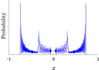
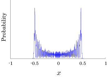
Probability disribution †
The probability that the walker can be observed at position  at time
  is defined by
![\[ \mathbb{P}(X_t=x)= ||\psi_t(x)||^2,\]](../image/equation/ae1a4d79fde5d7404445014dfe67b7e53b05b2f18ce46f0ada0bd65ba151.png "\[ \mathbb{P}(X_t=x)= ||\psi_t(x)||^2,\]")
where  is a random variable and denotes the position of the quantum walker.
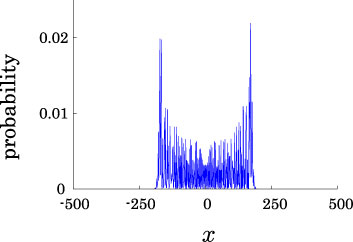
- Example
- Quantum walk v.s. Random walk
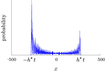
Limit theorem †
For complex numbers  , we take initial conditions to be
![\[ \psi_0(x)=\left\{\begin{array}{ll} {}^T[\alpha,\beta]&(x=0),\\ {}^T[0,0]&(x\neq 0), \end{array}\right.\]](../image/equation/10df1f4f626e49be8353d0b7e3eff6d43b05b2f18ce46f0ada0bd65ba151.png "\[ \psi_0(x)=\left\{\begin{array}{ll} {}^T[\alpha,\beta]&(x=0),\\ {}^T[0,0]&(x\neq 0), \end{array}\right.\]")
under the condition  . The symbol
  means the transposed operator.
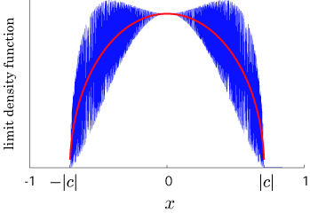
If we assume that the unitary matrix  satisfies the condition
  , then we have
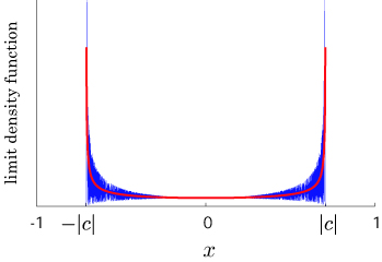
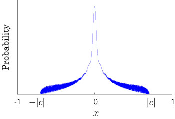
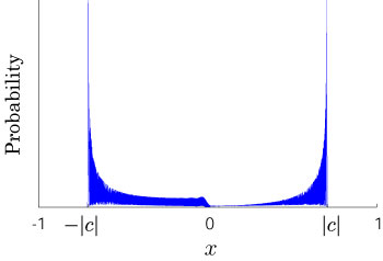
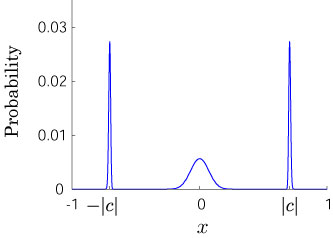
![\[ \lim_{t\to\infty} \mathbb{P}\left(\frac{X_t}{t} \leq x\right)=\int_{-\infty}^{x} f(y)\,I_{(-|a|,|a|)}(y)\,dy,\]](../image/equation/51b3e2590f1159fccd090a207fcde52a3b05b2f18ce46f0ada0bd65ba151.png "\[ \lim_{t\to\infty} \mathbb{P}\left(\frac{X_t}{t} \leq x\right)=\int_{-\infty}^{x} f(y)\,I_{(-|a|,|a|)}(y)\,dy,\]")
where
![\[ f(x)=\frac{\sqrt{1-|a|^2}}{\pi(1-x^2)\sqrt{|a|^2-x^2}}\left\{1-\left(|\alpha|^2-|\beta|^2+\frac{a\alpha\overline{b\beta}+\overline{a\alpha}b\beta}{|a|^2}\right)x\right\},\]](../image/equation/2042de8a478c46e344743ab6baa8ee6a3b05b2f18ce46f0ada0bd65ba151.png "\[ f(x)=\frac{\sqrt{1-|a|^2}}{\pi(1-x^2)\sqrt{|a|^2-x^2}}\left\{1-\left(|\alpha|^2-|\beta|^2+\frac{a\alpha\overline{b\beta}+\overline{a\alpha}b\beta}{|a|^2}\right)x\right\},\]")
and
![\[ I_{A}(x)=\left\{\begin{array}{cl} 1&(x\in A), \\ 0& (x\notin A). \end{array}\right.\]](../image/equation/2e44a8581ee2d8647feb83d559268df83b05b2f18ce46f0ada0bd65ba151.png "\[ I_{A}(x)=\left\{\begin{array}{cl} 1&(x\in A), \\ 0& (x\notin A). \end{array}\right.\]")
- Example
In the case of a simple random walk, we have
![\[ \lim_{t\to\infty} \mathbb{P}\left(\frac{X_t}{\sqrt{t}} \leq x\right)=\int_{-\infty}^{x} f(y)\,dy,\]](../image/equation/fac9de558c57ddc938f3974708cd38043b05b2f18ce46f0ada0bd65ba151.png "\[ \lim_{t\to\infty} \mathbb{P}\left(\frac{X_t}{\sqrt{t}} \leq x\right)=\int_{-\infty}^{x} f(y)\,dy,\]")
where
![\[ f(x)=\frac{1}{\sqrt{2\pi}}\,e^{-x^2/2}.\]](../image/equation/13c8a3d720d45659f2635ab75d7ec8fc3b05b2f18ce46f0ada0bd65ba151.png "\[ f(x)=\frac{1}{\sqrt{2\pi}}\,e^{-x^2/2}.\]")
Continuous-time quantum walk on the line †
Probability amplitude †
The whole system of a continuous-time quantum walk on the line  is also described by probability amplitudes.
The probability amplitude at position at time
is also described by probability amplitudes.
The probability amplitude at position at time  is expressed as a complex number
 ") , as shown in the following figure.
, as shown in the following figure.
Time evolution †
The time evolution is defined by a discrete-space Schrödinger equation,
![\[ i\frac{d\Psi_t(x)}{dt}=-\nu\left\{\Psi_t(x-1)-2\Psi_t(x)+\Psi_t(x+1)\right\},\]](../image/equation/c15a5c6a2ab58466c9fbb2d46f5db92f3b05b2f18ce46f0ada0bd65ba151.png "\[ i\frac{d\Psi_t(x)}{dt}=-\nu\left\{\Psi_t(x-1)-2\Psi_t(x)+\Psi_t(x+1)\right\},\]")
where  , and
, and  is a positive constant.
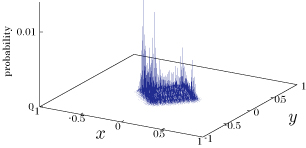
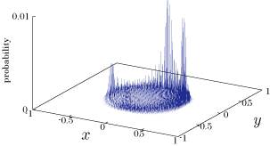
Probability distribution †
The quantum walker can be observed at position at time with probability
![\[ \mathbb{P}(X_t=x)= |\Psi_t(x)|^2.\]](../image/equation/b9b9a797296a84dcb8c2d0a69906dcfa3b05b2f18ce46f0ada0bd65ba151.png "\[ \mathbb{P}(X_t=x)= |\Psi_t(x)|^2.\]")
- Example
Limit theorem †
We take the initial conditions
![\[ \psi_0(x)=\left\{\begin{array}{ll} 1&(x=0),\\ 0&(x\neq 0). \end{array}\right.\]](../image/equation/32e0ae702d82531c5726e1720dc1caef3b05b2f18ce46f0ada0bd65ba151.png "\[ \psi_0(x)=\left\{\begin{array}{ll} 1&(x=0),\\ 0&(x\neq 0). \end{array}\right.\]")
Then we have
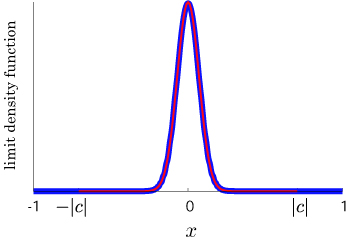
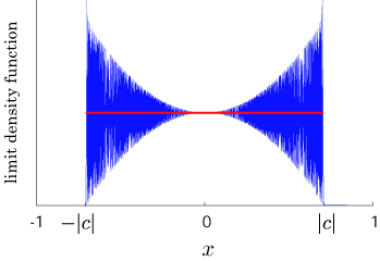
![\[ \lim_{t\rightarrow\infty}\mathbb{P}\left(\frac{X_t}{t}\leq x\right)=\int_{-\infty}^x f(y) \,I_{(-2\nu,2\nu)}(y)\,dy,\]](../image/equation/c88d5d472c558b89eb1f3715e6826f823b05b2f18ce46f0ada0bd65ba151.png "\[ \lim_{t\rightarrow\infty}\mathbb{P}\left(\frac{X_t}{t}\leq x\right)=\int_{-\infty}^x f(y) \,I_{(-2\nu,2\nu)}(y)\,dy,\]")
where
![\[ f(x)=\frac{1}{\pi\sqrt{(2\nu)^2-x^2}},\]](../image/equation/4b488a1e83f753063a4784eac056e38c3b05b2f18ce46f0ada0bd65ba151.png "\[ f(x)=\frac{1}{\pi\sqrt{(2\nu)^2-x^2}},\]")
and
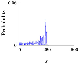
- Example
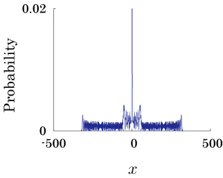
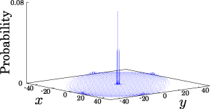
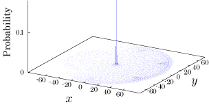
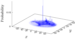
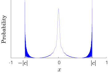
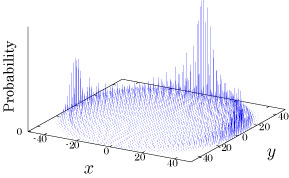
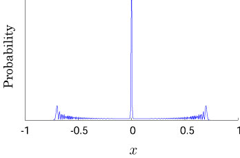
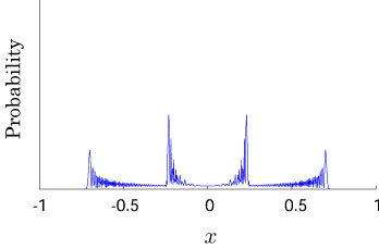
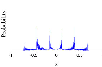
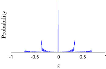
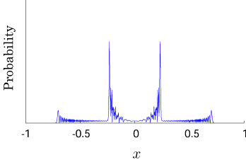
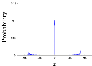
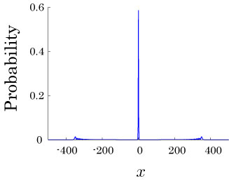
Interesting probability distributions of quantum walks †
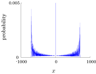
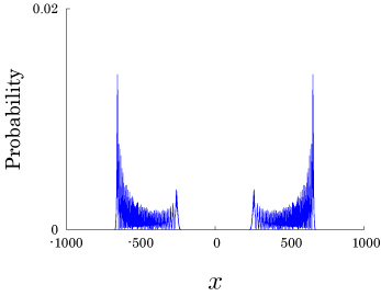
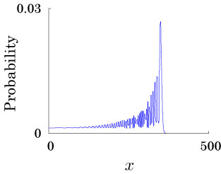
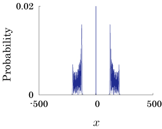
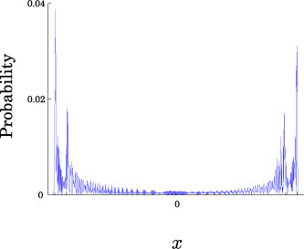
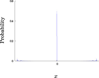
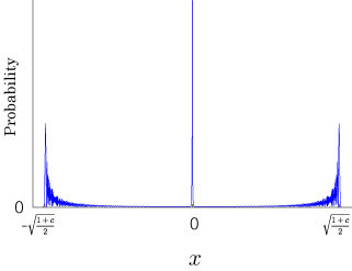
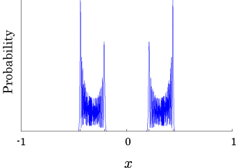
QIC, 15(13&14), 1248-1258 (2015)
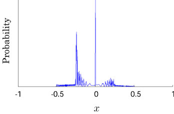
QIC, 10(11&12), 1004-1017 (2010)
IWNC 2009 Proc. ICT, 2, 226-235 (2010)
See also †
Further reading †
- Julia Kempe (2003). Quantum random walks – an introductory overview. Contemporary Physics 44 (4): 307–327. DOI:10.1080/00107151031000110776.
- Viv Kendon (2007). Decoherence in quantum walks – a review. Mathematical Structures in Computer Science 17 (6): 1169–1220. DOI:10.1017/S0960129507006354.
- Norio Konno (2008). Quantum Walks. Volume 1954 of Lecture Notes in Mathematics. Springer-Verlag, (Heidelberg) pp. 309–452. DOI:10.1007/978-3-540-69365-9.
- Salvador Elías Venegas-Andraca (2008). Quantum Walks for Computer Scientists. Morgan & Claypool Publishers. DOI:10.2200/S00144ED1V01Y200808QMC001.
- Salvador Elías Venegas-Andraca (2012). Quantum walks: a comprehensive review. Quantum Information Processing 11 (5): 1015–1106. DOI:10.1007/s11128-012-0432-5.